
In enterprise networks, the capacity problem usually begins as an invisible behavior change well before any link saturates. The backup link kicks in, east-west flows shift to other paths, the backup window stretches, and latency starts producing small spikes. Despite that, many teams still monitor backbone capacity at the level of “interface utilization percentage.” Yet backbone planning must be done by reading not just bandwidth but also traffic class, growth pattern, and resilience scenario together.
Why is classical percentage-based monitoring insufficient?
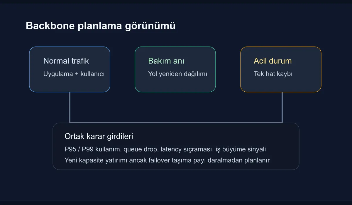
Because backbone links rarely carry steady, uniform traffic. During the day, application traffic dominates; at night, backup and replication; during a crisis, failover flows. The same average utilization figure can mean three very different risk profiles.
That is why the first step of capacity planning is to separate the main classes of traffic:
- User and application traffic
- Data replication and batch copy
- Management and observability flows
- Backup paths that activate during a disaster
Looking only at total Mbps lets these layers hide each other.
What inputs build a healthy model?
For backbone capacity planning, I find it useful to read four data sources together:
- P95 and P99 interface utilization
- Time-of-day pattern by traffic class
- Alternate-path load during failover or maintenance
- Volume drivers tied to business growth
Item three is especially critical. Many network designs look comfortable in the normal state but suddenly produce a bottleneck when a single uplink is lost. Backbone planning cannot be done from the happy-day graph alone.
How should the capacity threshold be defined?
Organizations generally operate with a single threshold like seventy or eighty percent. This is practical but incomplete. A better method is to define three thresholds per traffic class:
- The normal-operation threshold
- The maintenance and rerouting threshold
- The emergency-carrying threshold
For example, if everyday utilization on a data center backbone is forty-five percent but rises to seventy-eight percent on the loss of a single spine, the system is healthy today but fragile from a growth standpoint. Without making this distinction, investment is always late.
Why does the observability layer have a direct effect?
Because capacity planning is not a report on the past but a warning about the future. If NetFlow, sFlow, queue drop, interface error, and latency measurements are not read in a single view, the problem only becomes visible once user impact has formed. In particular, these signals must be considered together:
- Microburst behavior growing on the same path
- Queue discards correlated with rising application timeouts
- Route changes and throughput differences during failover tests
- Hours when backup and observability flows overlap
Without that visibility, the capacity issue becomes a bottleneck noticed late not just by the network team but by the entire platform.
How does the decision moment arrive in enterprise architecture?
The decision to invest should not wait for the port to fill completely. A more accurate approach is to see where the safety margin drops in specific scenarios and decide on that basis. I find these questions effective:
- On the loss of a single uplink, which workload breaks first?
- Over the next two quarters, which project will permanently lift traffic?
- Is the QoS definition really protecting the critical flows?
- Is new capacity the right investment, or is better traffic separation?
These questions move backbone planning out of a device-count exercise and into the level of architectural decisions.
Conclusion
A backbone capacity planning model for enterprise networks is more than reading interface graphs. When you bring traffic classes, failover behavior, business growth, and observability signals into the same frame, investment decisions become earlier and more defensible. In backbone design, real resilience starts not after the link fills, but at the moment you build the right model before it does.